Clustering of coral reef soundscape

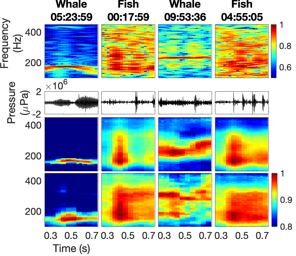
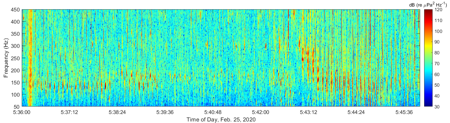
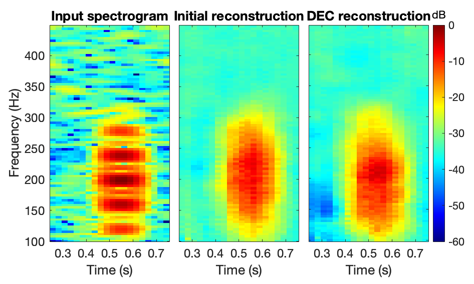
I customized a deep embedded clustering (DEC) algorithm to separate fish calls and whale song in spectrograms of coral reef ambient noise (Figure 1). These data were collected in February to March 2020 near Kona Bay (Figure 2) by a team including myself.

Figure 1: A time-frequency image, or spectrogram, of about 10 minutes of coral reef noise. Red features are louder, usually representing fish or whale sounds. Blue sections are more quiet.

Figure 2: Photo of Kona Bay near the field site.

1 Data Generation and Processing

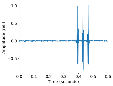
Fish communicate with series of pulses generated by their swim bladders. We simulate pulses with a Gaussian-modulated sinusoid of N random pulses and a center frequency f_c based on observations of real fish pulses. The pulses are randomly offset and spaced at a random dt. The random seed and reference phase are fixed, which guarantees we are always generating the same dataset!

rng(seed)
iphase = rd.rand(1)
for ii in np.arange(N):
    ⋮
    x = x+np.sin(-2*np.pi*(fc*(t-dt*ii-offset)+iphase))*np.exp(-a*(t-dt*ii-offset)**2)

The discrete fourier transform (DFT) generates a spectrogram. The image is created by using the magnitude (absolute value). We use the same DFT length for fish calls and whale song, aiming for a happy medium between good time resolution and frequency resolution of both.

\xrightarrow[]{\text{DFT}}

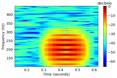
Humpback whales songs are frequency-modulated sinusoids, also called quadratic sweeps. The length of the sweep T, start frequency f_0, and bandwidth df are based on observed data and previous studies. The call can have an upsweep (df > 0) or a downsweep (df < 0).

rng(seed)
delta = (t>offset)*(t<(offset+T))
x = delta*np.sin(-2*np.pi*(df/(T**2)/3*(t-offset)**3 + f0*(t-offset) + rd.rand(1)))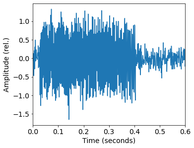

\xrightarrow[]{\text{DFT}}

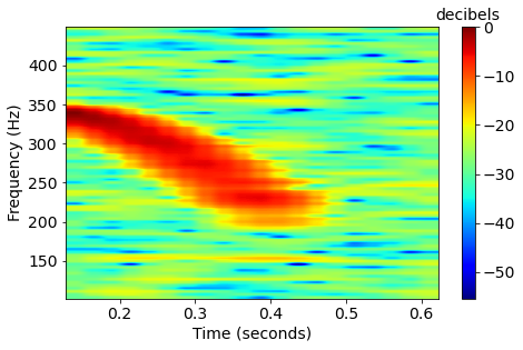
Both signals are normalized to their maximum, and then Gaussian noise is added with a random signal-to-noise ratio (SNR) using \sigma.

x = x/np.max(np.abs(x[:]))
xn = x+sigma*rd.randn(x.shape[-1])

The reconstructed images allow us to test the class ratios on the DEC model, and to use transfer learning from the simulated data to real data.

2 Deep clustering model

The DEC uses a convolutional auto-encoder (CAE, see Figure 3) to learn low-dimensional representations of the image, also called kernels. A loss function (L_1) is used to accurately regenerate the input image from these kernels. Then, I retrained the CAE with a clustering penalty (L_2) that encourages grouping of similar kernels.

Figure 3: A diagram of the deep clustering model workflow and layer sizes.

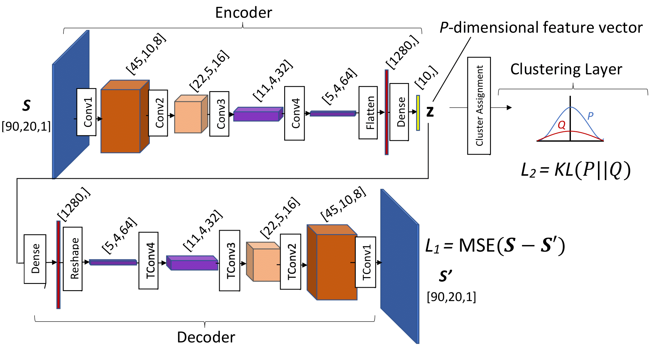
The cluster loss selected for this project was the KL is the Kullback-Leibler divergence,

KL(P||Q) = \sum_n \sum_k p_{nk} \log \left(\frac{p_{nk}}{q_{nk}} \right)

q_{nk} is the empirical Student’s t-distribution of the kernel variables around their cluster means, which are initialized with K-means. p_{nk} is the weighted squared distribution of q_{nk}, and it puts more penalty on kernels that are further from their cluster center, causing them to have larger adjustments toward the center during training.

More details can be found in our paper:

E. Ozanich, A. Thode, P. Gerstoft, L. A. Freeman, and S. Freeman, “Deep embedded clustering of coral reef bioacoustics,” J. Acoust. Soc. Am. 149 (2021): 2587–2601.

Figure 4: Example simulated fish call, its reconstruction from kernels, and the reconstruction after applying clustering.

3 Results

We look at the results of the DEC method after simulating 100 different datasets. The known labels from the simulations were used to test the model performance.

Three cases were considered: equal-sized groups (classes) of whale song and fish calls (a-c), inequal-sized classes of whale song and fish call (d-f), and equal-sized clsases of whale song, fish call, and whale song overlaying fish call (g-i). Since we suspect many more fish calls than whale song after observing the experimental data, we test the effect of inequal class size on the model.

Figure 5: t-SNE visualization of clustering performance for simulated data using (a-c) two equally sized classes, (d-f) two imbalanced classes, and (g-i) three classes, using manual labeling, Gaussian mixture models on the latent features, or the DEC pipeline.

Observing that DEC does not perform well for inequal class sizes, we added the Gaussian mixture means (GMM) method for comparison. GMM was applied directly to the kernels from CAE without additional training of the DEC. The DEC algorithm uses the K-means assumption of equi-distant clusters (fixed-variance Gaussians), whereas GMM learns the variance and the cluster means, allowing it to optimize cluster sizes.

Figure 6: t-SNE visualization of clustering performance for real coral reef data using (a) manual labels, (b) k-means clustering, (c) Gaussian mixture models, and (d) the DEC pipeline.

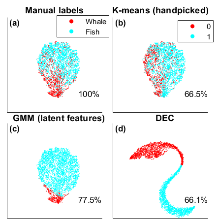
Using some hand-labeled events detected in the experiment data, we show that the GMM does perform better than DEC due to the class imbalance in the real data. Unlike curated data, these raw data contain multiple, often overlapping, signals with varying SNR, including unknown signals not accounted for. Additional array processing and human labeling is needed to raise the accuracy from 77% to >90%.

Figure 7: Examples of real coral reef spectrograms used as inputs for the CNN and DEC feature extraction and clustering pipeline.